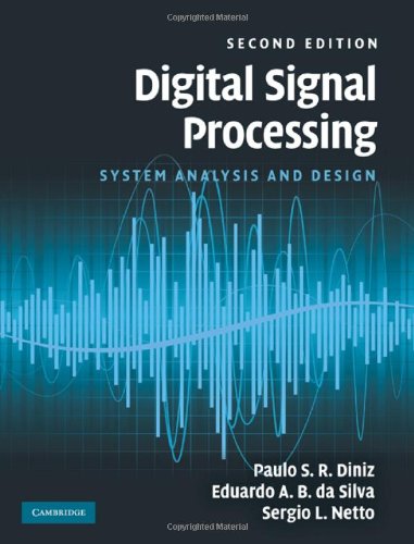
Digital Signal Processing System Analysis and Design 2nd Edition by Paulo Diniz, Eduardo da Silva, Sergio Netto 0521887755 9780521887755
$50.00 Original price was: $50.00.$35.00Current price is: $35.00.
Digital Signal Processing System Analysis and Design 2nd Edition by Paulo Diniz, Eduardo da Silva, Sergio Netto – Ebook PDF Instant Download/Delivery: 0521887755, 9780521887755
Full download Digital Signal Processing System Analysis and Design 2nd Edition after payment

Product details:
ISBN 10: 0521887755
ISBN 13: 9780521887755
Author: Paulo S. R. Diniz, Eduardo A. B. da Silva, Sergio L. Netto
This new, fully-revised edition covers all the major topics of digital signal processing (DSP) design and analysis in a single, all-inclusive volume, interweaving theory with real-world examples and design trade-offs. Building on the success of the original, this edition includes new material on random signal processing, a new chapter on spectral estimation, greatly expanded coverage of filter banks and wavelets, and new material on the solution of difference equations. Additional steps in mathematical derivations make them easier to follow, and an important new feature is the do-it-yourself section at the end of each chapter, where readers get hands-on experience of solving practical signal processing problems in a range of MATLAB experiments. With 120 worked examples, 20 case studies, and almost 400 homework exercises, the book is essential reading for anyone taking DSP courses. Its unique blend of theory and real-world practical examples also makes it an ideal reference for practitioners.
Table of contents:
1 Discrete-time signals and systems
1.1 Introduction
1.2 Discrete-time signals
1.3 Discrete-time systems
1.3.1 Linearity
1.3.2 Time invariance
1.3.3 Causality
1.3.4 Impulse response and convolution sums
1.3.5 Stability
1.4 Difference equations and time-domain response
1.4.1 Recursive × nonrecursive systems
1.5 Solving difference equations
1.5.1 Computing impulse responses
1.6 Sampling of continuous-time signals
1.6.1 Basic principles
1.6.2 Sampling theorem
1.7 Random signals
1.7.1 Random variable
1.7.2 Random processes
1.7.3 Filtering a random signal
1.8 Do-it-yourself: discrete-time signals and systems
Experiment 1.1
Experiment 1.2
Experiment 1.3
1.9 Discrete-time signals and systems with MATLAB
1.10 Summary
1.11 Exercises
2 The z and Fourier transforms
2.1 Introduction
2.2 Definition of the z transform
2.3 Inverse z transform
2.3.1 Computation based on residue theorem
2.3.2 Computation based on partial-fraction expansions
2.3.3 Computation based on polynomial division
2.3.4 Computation based on series expansion
2.4 Properties of the z transform
2.4.1 Linearity
2.4.2 Time reversal
2.4.3 Time-shift theorem
2.4.4 Multiplication by an exponential
2.4.5 Complex differentiation
2.4.6 Complex conjugation
2.4.7 Real and imaginary sequences
2.4.8 Initial-value theorem
2.4.9 Convolution theorem
2.4.10 Product of two sequences
2.4.11 Parseval’s theorem
2.4.12 Table of basic z transforms
2.5 Transfer functions
2.6 Stability in the z domain
2.7 Frequency response
2.8 Fourier transform
2.9 Properties of the Fourier transform
2.9.1 Linearity
2.9.2 Time reversal
2.9.3 Time-shift theorem
2.9.4 Multiplication by a complex exponential (frequency shift, modulation)
2.9.5 Complex differentiation
2.9.6 Complex conjugation
2.9.7 Real and imaginary sequences
2.9.8 Symmetric and antisymmetric sequences
2.9.9 Convolution theorem
2.9.10 Product of two sequences
2.9.11 Parseval’s theorem
2.10 Fourier transform for periodic sequences
2.11 Random signals in the transform domain
2.11.1 Power spectral density
2.11.2 White noise
2.12 Do-it-yourself: the z and Fourier transforms
Experiment 2.1
Experiment 2.2
Experiment 2.3
2.13 The z and Fourier transforms with MATLAB
2.14 Summary
2.15 Exercises
3 Discrete transforms
3.1 Introduction
3.2 Discrete Fourier transform
3.3 Properties of the DFT
3.3.1 Linearity
3.3.2 Time reversal
3.3.3 Time-shift theorem
3.3.4 Circular frequency-shift theorem (modulation theorem)
3.3.5 Circular convolution in time
3.3.6 Correlation
3.3.7 Complex conjugation
3.3.8 Real and imaginary sequences
3.3.9 Symmetric and antisymmetric sequences
3.3.10 Parseval’s theorem
3.3.11 Relationship between the DFT and the z transform
3.4 Digital filtering using the DFT
3.4.1 Linear and circular convolutions
3.4.2 Overlap-and-add method
3.4.3 Overlap-and-save method
3.5 Fast Fourier transform
3.5.1 Radix-2 algorithm with decimation in time
3.5.2 Decimation in frequency
3.5.3 Radix-4 algorithm
3.5.4 Algorithms for arbitrary values of N
3.5.5 Alternative techniques for determining the DFT
3.6 Other discrete transforms
3.6.1 Discrete transforms and Parseval’s theorem
3.6.2 Discrete transforms and orthogonality
3.6.3 Discrete cosine transform
3.6.4 A family of sine and cosine transforms
3.6.5 Discrete Hartley transform
3.6.6 Hadamard transform
3.6.7 Other important transforms
Wavelet transforms
Karhunen–Loève transform
3.7 Signal representations
3.7.1 Laplace transform
3.7.2 The z transform
3.7.3 Fourier transform (continuous time)
3.7.4 Fourier transform (discrete time)
3.7.5 Fourier series
3.7.6 Discrete Fourier transform
3.8 Do-it-yourself: discrete transforms
Experiment 3.1
Experiment 3.2
3.9 Discrete transforms with MATLAB
3.10 Summary
3.11 Exercises
4 Digital filters
4.1 Introduction
4.2 Basic structures of nonrecursive digital filters
4.2.1 Direct form
4.2.2 Cascade form
4.2.3 Linear-phase forms
4.3 Basic structures of recursive digital filters
4.3.1 Direct forms
4.3.2 Cascade form
4.3.3 Parallel form
4.4 Digital network analysis
4.5 State-space description
4.6 Basic properties of digital networks
4.6.1 Tellegen’s theorem
4.6.2 Reciprocity
4.6.3 Interreciprocity
4.6.4 Transposition
4.6.5 Sensitivity
4.7 Useful building blocks
4.7.1 Second-order building blocks
4.7.2 Digital oscillators
4.7.3 Comb filter
4.8 Do-it-yourself: digital filters
Experiment 4.1
4.9 Digital filter forms with MATLAB
4.10 Summary
4.11 Exercises
5 FIR filter approximations
5.1 Introduction
5.2 Ideal characteristics of standard filters
5.2.1 Lowpass, highpass, bandpass, and bandstop filters
5.2.2 Differentiators
5.2.3 Hilbert transformers
5.2.4 Summary
5.3 FIR filter approximation by frequency sampling
5.4 FIR filter approximation with window functions
5.4.1 Rectangular window
5.4.2 Triangular windows
5.4.3 Hamming and Hann windows
5.4.4 Blackman window
5.4.5 Kaiser window
5.4.6 Dolph–Chebyshev window
5.5 Maximally flat FIR filter approximation
5.6 FIR filter approximation by optimization
5.6.1 Weighted least-squares method
5.6.2 Chebyshev method
5.6.3 WLS–Chebyshev method
5.7 Do-it-yourself: FIR filter approximations
Experiment 5.1
Experiment 5.2
5.8 FIR filter approximation with MATLAB
5.9 Summary
5.10 Exercises
6 IIR filter approximations
6.1 Introduction
6.2 Analog filter approximations
6.2.1 Analog filter specification
6.2.2 Butterworth approximation
6.2.3 Chebyshev approximation
6.2.4 Elliptic approximation
6.2.5 Frequency transformations
6.3 Continuous-time to discrete-time transformations
6.3.1 Impulse-invariance method
6.3.2 Bilinear transformation method
6.4 Frequency transformation in the discrete-time domain
6.4.1 Lowpass-to-lowpass transformation
6.4.2 Lowpass-to-highpass transformation
6.4.3 Lowpass-to-bandpass transformation
6.4.4 Lowpass-to-bandstop transformation
6.4.5 Variable-cutoff filter design
6.5 Magnitude and phase approximation
6.5.1 Basic principles
6.5.2 Multivariable function minimization method
6.5.3 Alternative methods
6.6 Time-domain approximation
6.6.1 Approximate approach
6.7 Do-it-yourself: IIR filter approximations
Experiment 6.1
Experiment 6.2
6.8 IIR filter approximation with MATLAB
6.9 Summary
6.10 Exercises
7 Spectral estimation
7.1 Introduction
7.2 Estimation theory
7.3 Nonparametric spectral estimation
7.3.1 Periodogram
7.3.2 Periodogram variations
7.3.3 Minimum-variance spectral estimator
7.4 Modeling theory
7.4.1 Rational transfer-function models
7.4.2 Yule–Walker equations
7.5 Parametric spectral estimation
7.5.1 Linear prediction
7.5.2 Covariance method
7.5.3 Autocorrelation method
7.5.4 Levinson–Durbin algorithm
7.5.5 Burg’s method
7.5.6 Relationship of the Levinson–Durbin algorithm to a lattice structure
7.6 Wiener filter
7.7 Other methods for spectral estimation
7.8 Do-it-yourself: spectral estimation
Experiment 7.1
Experiment 7.2
7.9 Spectral estimation with MATLAB
7.10 Summary
7.11 Exercises
8 Multirate systems
8.1 Introduction
8.2 Basic principles
8.3 Decimation
8.4 Interpolation
8.4.1 Examples of interpolators
8.5 Rational sampling-rate changes
8.6 Inverse operations
8.7 Noble identities
8.8 Polyphase decompositions
8.9 Commutator models
8.10 Decimation and interpolation for efficient filter implementation
8.10.1 Narrowband FIR filters
8.10.2 Wideband FIR filters with narrow transition bands
8.11 Overlapped block filtering
8.11.1 Nonoverlapped case
8.11.2 Overlapped input and output
8.11.3 Fast convolution structure I
8.11.4 Fast convolution structure II
8.12 Random signals in multirate systems
8.12.1 Interpolated random signals
8.12.2 Decimated random signals
8.13 Do-it-yourself: multirate systems
Experiment 8.1
8.14 Multirate systems with MATLAB
8.15 Summary
8.16 Exercises
9 Filter banks
9.1 Introduction
9.2 Filter banks
9.2.1 Decimation of a bandpass signal
9.2.2 Inverse decimation of a bandpass signal
9.2.3 Critically decimated M-band filter banks
9.3 Perfect reconstruction
9.3.1 M-band filter banks in terms of polyphase components
9.3.2 Perfect reconstruction M-band filter banks
9.4 Analysis of M-band filter banks
9.4.1 Modulation matrix representation
9.4.2 Time-domain analysis
9.4.3 Orthogonality and biorthogonality in filter banks
9.4.3.1 Orthogonality in the z transform domain
9.4.4 Transmultiplexers
9.5 General two-band perfect reconstruction filter banks
9.6 QMF filter banks
9.7 CQF filter banks
9.8 Block transforms
9.9 Cosine-modulated filter banks
9.9.1 The optimization problem in the design of cosine-modulated filter banks
9.10 Lapped transforms
9.10.1 Fast algorithms and biorthogonal LOT
9.10.2 Generalized LOT
9.11 Do-it-yourself: filter banks
Experiment 9.1
Experiment 9.2
9.12 Filter banks with MATLAB
9.13 Summary
9.14 Exercises
10 Wavelet transforms
10.1 Introduction
10.2 Wavelet transforms
10.2.1 Hierarchical filter banks
10.2.2 Wavelets
10.2.3 Scaling functions
10.3 Relation between x(t) and x(n)
10.4 Wavelet transforms and time–frequency analysis
10.4.1 The short-time Fourier transform
10.4.2 The continuous-time wavelet transform
10.4.3 Sampling the continuous-time wavelet transform: the discrete wavelet transform
10.5 Multiresolution representation
10.5.1 Biorthogonal multiresolution representation
10.6 Wavelet transforms and filter banks
10.6.1 Relations between the filter coefficients
10.7 Regularity
10.7.1 Additional constraints imposed on the filter banks due to the regularity condition
10.7.2 A practical estimate of regularity
10.7.3 Number of vanishing moments
10.8 Examples of wavelets
10.9 Wavelet transforms of images
10.10 Wavelet transforms of finite-length signals
10.10.1 Periodic signal extension
10.10.2 Symmetric signal extensions
10.11 Do-it-yourself: wavelet transforms
Experiment 10.1
Experiment 10.2
10.12 Wavelets with MATLAB
10.13 Summary
10.14 Exercises
11 Finite-precision digital signal processing
11.1 Introduction
11.2 Binary number representation
11.2.1 Fixed-point representations
11.2.1.1 Sign-magnitude representation
11.2.1.2 One’s-complement representation
11.2.1.3 Two’s-complement representation
11.2.2 Signed power-of-two representation
11.2.3 Floating-point representation
11.3 Basic elements
11.3.1 Properties of the two’s-complement representation
11.3.2 Serial adder
11.3.3 Serial multiplier
11.3.4 Parallel adder
11.3.5 Parallel multiplier
11.4 Distributed arithmetic implementation
11.5 Product quantization
11.6 Signal scaling
11.7 Coefficient quantization
11.7.1 Deterministic sensitivity criterion
11.7.2 Statistical forecast of the wordlength
11.8 Limit cycles
11.8.1 Granular limit cycles
11.8.2 Overflow limit cycles
11.8.3 Elimination of zero-input limit cycles
11.8.4 Elimination of constant-input limit cycles
11.8.5 Forced-response stability of digital filters with nonlinearities due to overflow
11.9 Do-it-yourself: finite-precision digital signal processing
Experiment 11.1
Experiment 11.2
11.10 Finite-precision digital signal processing with MATLAB
11.11 Summary
11.12 Exercises
12 Efficient FIR structures
12.1 Introduction
12.2 Lattice form
12.2.1 Filter banks using the lattice form
12.3 Polyphase form
12.4 Frequency-domain form
12.5 Recursive running sum form
12.6 Modified-sinc filter
12.7 Realizations with reduced number of arithmetic operations
12.7.1 Prefilter approach
12.7.2 Interpolation approach
12.7.3 Frequency-response masking approach
12.7.4 Quadrature approach
12.8 Do-it-yourself: efficient FIR structures
Experiment 12.1
12.9 Efficient FIR structures with MATLAB
12.10 Summary
12.11 Exercises
13 Efficient IIR structures
13.1 Introduction
13.2 IIR parallel and cascade filters
13.2.1 Parallel form
13.2.2 Cascade form
13.2.3 Error spectrum shaping
13.2.4 Closed-form scaling
13.3 State-space sections
13.3.1 Optimal state-space sections
13.3.2 State-space sections without limit cycles
13.4 Lattice filters
13.5 Doubly complementary filters
13.5.1 QMF filter bank implementation
13.6 Wave filters
13.6.1 Motivation
13.6.2 Wave elements
13.6.2.1 One-port elements
13.6.2.2 Voltage generalized immittance converter
13.6.2.3 Current generalized immittance converter
13.6.2.4 Transformer
13.6.2.5 Gyrator
13.6.2.6 Two-port adaptors
13.6.2.7 The n-port parallel adaptor
13.6.2.8 The n-port series adaptor
13.6.3 Lattice wave digital filters
13.7 Do-it-yourself: efficient IIR structures
Experiment 13.1
13.8 Efficient IIR structures with MATLAB
13.9 Summary
13.10 Exercises
People also search:
why digital signal processing
what is system in digital signal processing
how does digital signal processing work
what does digital signal processing mean
digital signal processing examples
Tags: Paulo Diniz, Eduardo da Silva, Sergio Netto, Processing


